图像的语义分割

图像的语义分割简单来说就是对于图像的每一个像素，都给出对应的类别，从而实现像素级别的分类。

运行环境

tensorflow2.0.0

[[数据集]] 介绍

[[Cityscapes]] 数据集

精细注释数据集包含 2975 张训练图片和 500 张验证图片。包含了街景图片和对应的标签，标签共 34 类。

数据集包含两部分 leftImg8bit 和 gtFine 文件夹，leftImg8bit 为原始图片，gtFine 为对应标签 Images 图像大小为 2048*1024， gtFine 是图像的分割图

[[U-Net]] 模型

U-Net 简介

U-Net 是一个非常知名的用来进行图像语义分割的深度卷积神经网络，刚开始主要是应用于医学图像处理方面

U-Net 和 FCN 非常的相似，U-Net 比 FCN 稍晚提出来，但都发表在 2015 年，和 FCN 相比，U-Net 的第一个特点是完全对称，也就是左边和右边是很类似的，而 FCN 的 decoder 相对简单，只用了一个 deconvolution 的操作，之后并没有跟上卷积结构。

第二个区别就是 skip connection，FCN 用的是加操作（summation），U-Net 用的是叠操作（concatenation）。这些都是细节，重点是它们的结构用了一个比较经典的思路，也就是编码和解码（encoder-decoder），早在 2006 年就被 Hinton 大神提出来发表在了 nature 上.

U-Net 网络结构

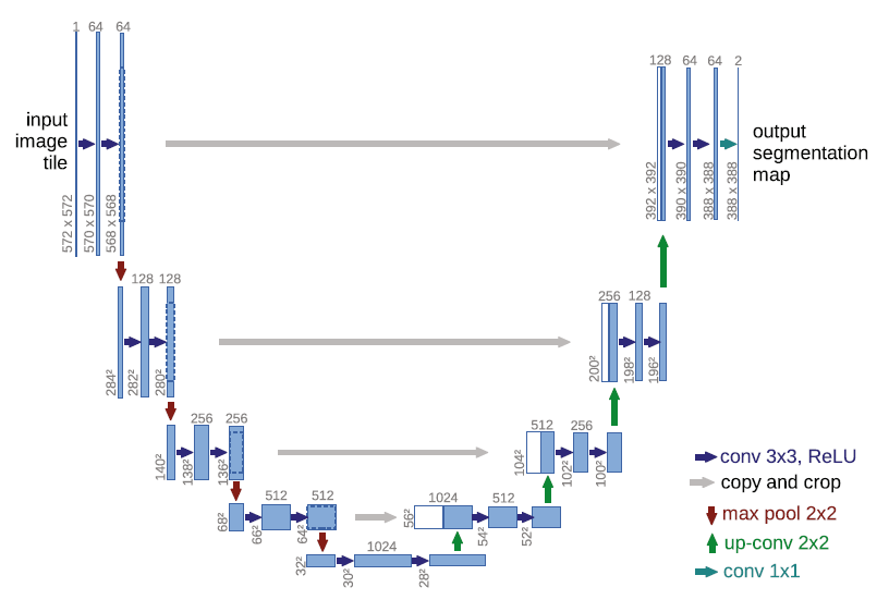
整个 U-Net 网络结构如图，类似于一个大大的 U 字母：首先进行 Conv+Pooling 下采样；然后 Deconv 反卷积进行上采样，crop 之前的低层 feature map，进行融合；然后再次上采样。重复这个过程，直到获得输出 388x388x2 的 feature map，最后经过 softmax 获得 output segment map。总体来说与 FCN 思路非常类似。

U-Net 特点

在小数据集上表现良好使用 tf.concat 进行叠加，与 [[FCN]] 的 tf.add 有区别

Tensorflow 代码

导入包

import tensorflow as tf
import matplotlib.pyplot as plt
import numpy as np
import os
import glob

加载打乱训练集

首先将需要训练与验证的图片路径都加载进来

# 获取数据路径列表 2975 张训练图片
# 图片大小 1024*2048
img = glob.glob (r"./dataset/leftImg8bit/train/*/*.png")
train_count = len (img)
# 标注列表
label = glob.glob (r"./dataset/gtFine/train/*/*_gtFine_labelIds.png")


# 测试集图片 500 张
img_val = glob.glob (r"./dataset/leftImg8bit/val/*/*.png")
label_val = glob.glob (r"./dataset/gtFine/val/*/*_gtFine_labelIds.png")
test_count = len (img_val)

# 将训练图片打乱
np.random.seed (2019)
# 创建长度为 image 图片数量的乱序列表
index = np.random.permutation (len (img))
img = np.array (img)[index]
label = np.array (label)[index]

定义加载变换函数

将图片转为 tensor 类型，并且且进行数据增强，引入随机裁剪与翻转

def read_png_image (path):
    # 训练集图片为彩色图片 channel 为 3
    img = tf.io.read_file (path)

    img = tf.image.decode_png (img, channels=3)
    return img


def read_png_label (path):
    # 验证集图片为灰度图片 channel 为 1
    img = tf.io.read_file (path)
    img = tf.image.decode_png (img, channels=1)
    return img


def crop_img (img, label):
    """ 图片随机裁剪

    将 img 与 label 通道合并，然后缩放，再进行随机分割
    """
    # [1024,2048,3]+[1024,2048,1]-> [1024,2048,4] 合并
    concat_img = tf.concat ([img, label], axis=-1)

    # 缩放 [1024,2048,4]-> [280,280,4]
    concat_img = tf.image.resize (
        concat_img, (280, 280), method=tf.image.ResizeMethod.NEAREST_NEIGHBOR)

    # 随机裁剪 [280,280,4]-> [256,256,4]
    crop_img = tf.image.random_crop (concat_img, size=[256, 256, 4])

    # 分割回来
    img, label = tf.split (
        crop_img, axis=-1, num_or_size_splits=[3, 1])
    return img, label


def normal_img (img, label):
    """ 图片归一化
    """
    img = tf.cast (img, tf.float32)
    label = tf.cast (label, tf.int32)
    img = img / 127.5 - 1  # 归一化到 [-1,1]
    return img, label


def load_train (img_path, label_path):
    """ 加载训练集

    引入随机翻转
    """
    # 读取
    img = read_png_image (img_path)
    label = read_png_label (label_path)

    # 裁剪
    img, label = crop_img (img, label)

    # 随机翻转
    if tf.random.uniform (()) > 0.5:
        img = tf.image.flip_left_right (img)
        label = tf.image.flip_left_right (label)

    return normal_img (img, label)


def load_val (img_path, label_path):
    """ 加载验证集

    不需要做裁剪但需要做 resize 到 [256,256]
    """
    img = read_png_image (img_path)
    label = read_png_label (label_path)
    img = tf.image.resize (img, (256, 256))
    label = tf.image.resize (label, (256, 256))

    return normal_img (img, label)

数据集配置

EPOCHS = 60
BATCH_SIZE = 32
BUFFER_SIZE = 300
# 数据库迭代一次需要的 step 数
steps_per_epoch = train_count // BATCH_SIZE
val_step = test_count // BATCH_SIZE


dataset_train = tf.data.Dataset.from_tensor_slices ((img, label))
dataset_val = tf.data.Dataset.from_tensor_slices ((img_val, label_val))


AUTOTUNE = tf.data.experimental.AUTOTUNE
dataset_train = dataset_train.map (
    load_train, num_parallel_calls=AUTOTUNE)  # 多线程自动判断
dataset_val = dataset_val.map (
    load_val, num_parallel_calls=AUTOTUNE)  # 多线程自动判断

# %% 数据集配置
# prefetch ()：GPU 练时 CPU 继续读取
dataset_train = dataset_train.cache ().repeat ().shuffle (
    BUFFER_SIZE).batch (BATCH_SIZE).prefetch (AUTOTUNE)

dataset_val = dataset_val.cache ().batch (BATCH_SIZE)

创建模型

对照 U-Net 模型搭建网络，为了图片大小在卷积过程中保持不变，需要进行零填充

def create_model ():
   inputs = tf.keras.layers.Input (shape=(256, 256, 3))

   # 下采样部分
   # [256,256,3]-> [256,256,64]
   x = tf.keras.layers.Conv2D (
       64, 3, padding="same", activation="relu")(inputs)
   x = tf.keras.layers.BatchNormalization ()(x)
   x = tf.keras.layers.Conv2D (64, 3, padding="same", activation="relu")(x)
   x = tf.keras.layers.BatchNormalization ()(x)

   # [256,256,64]-> [128,128,64]
   x1 = tf.keras.layers.MaxPooling2D (padding="same")(x)
   # [128,128,64]-> [128,128,128]
   x1 = tf.keras.layers.Conv2D (128, 3, padding="same", activation="relu")(x1)
   x1 = tf.keras.layers.BatchNormalization ()(x1)
   x1 = tf.keras.layers.Conv2D (128, 3, padding="same", activation="relu")(x1)
   x1 = tf.keras.layers.BatchNormalization ()(x1)

   # [128,128,128]-> [64,64,128]
   x2 = tf.keras.layers.MaxPooling2D (padding="same")(x1)
   # [64,64,128]-> [64,64,256]
   x2 = tf.keras.layers.Conv2D (256, 3, padding="same", activation="relu")(x2)
   x2 = tf.keras.layers.BatchNormalization ()(x2)
   x2 = tf.keras.layers.Conv2D (256, 3, padding="same", activation="relu")(x2)
   x2 = tf.keras.layers.BatchNormalization ()(x2)

   # [64,64,256]-> [64,64,512]
   x3 = tf.keras.layers.MaxPooling2D (padding="same")(x2)
   # [64,64,512]-> [32,32,512]
   x3 = tf.keras.layers.Conv2D (512, 3, padding="same", activation="relu")(x3)
   x3 = tf.keras.layers.BatchNormalization ()(x3)
   x3 = tf.keras.layers.Conv2D (512, 3, padding="same", activation="relu")(x3)
   x3 = tf.keras.layers.BatchNormalization ()(x3)

   # [32,32,512]-> [16,16,512]
   x4 = tf.keras.layers.MaxPooling2D (padding="same")(x3)
   # [16,16,512]-> [16,16,1024]
   x4 = tf.keras.layers.Conv2D (1024, 3, padding="same", activation="relu")(x4)
   x4 = tf.keras.layers.BatchNormalization ()(x4)
   x4 = tf.keras.layers.Conv2D (1024, 3, padding="same", activation="relu")(x4)
   x4 = tf.keras.layers.BatchNormalization ()(x4)

   # 上采样部分
   # [16,16,1024]-> [32,32,512] strides=2: 放大两倍
   x5 = tf.keras.layers.Conv2DTranspose (
       512, 2, strides=2, padding="same", activation="relu")(x4)
   x5 = tf.keras.layers.BatchNormalization ()(x5)

   # [32,32,512]+[32,32,512]-> [32,32,1024]
   x6 = tf.concat ([x3, x5], axis=-1)
   # [32,32,1024]-> [32,32,512]
   x6 = tf.keras.layers.Conv2D (512, 3, padding="same", activation="relu")(x6)
   x6 = tf.keras.layers.BatchNormalization ()(x6)
   x6 = tf.keras.layers.Conv2D (512, 3, padding="same", activation="relu")(x6)
   x6 = tf.keras.layers.BatchNormalization ()(x6)

   # [32,32,512]-> [64,64,256]
   x7 = tf.keras.layers.Conv2DTranspose (
       256, 2, strides=2, padding="same", activation="relu")(x6)
   x7 = tf.keras.layers.BatchNormalization ()(x7)

   # [64,64,256]+[64,64,256]-> [64,64,512]
   x8 = tf.concat ([x2, x7], axis=-1)
   # [64,64,512]-> [64,64,256]
   x8 = tf.keras.layers.Conv2D (256, 3, padding="same", activation="relu")(x8)
   x8 = tf.keras.layers.BatchNormalization ()(x8)
   x8 = tf.keras.layers.Conv2D (256, 3, padding="same", activation="relu")(x8)
   x8 = tf.keras.layers.BatchNormalization ()(x8)

   # [64,64,256]-> [128,128,128]
   x9 = tf.keras.layers.Conv2DTranspose (
       128, 2, strides=2, padding="same", activation="relu")(x8)
   x9 = tf.keras.layers.BatchNormalization ()(x9)

   # [128,128,128]+[128,128,128]-> [128,128,256]
   x10 = tf.concat ([x1, x9], axis=-1)
   # [128,128,256]-> [128,128,128]
   x10 = tf.keras.layers.Conv2D (
       128, 3, padding="same", activation="relu")(x10)
   x10 = tf.keras.layers.BatchNormalization ()(x10)
   x10 = tf.keras.layers.Conv2D (
       128, 3, padding="same", activation="relu")(x10)
   x10 = tf.keras.layers.BatchNormalization ()(x10)

   # [128,128,128]-> [256,256,64]
   x11 = tf.keras.layers.Conv2DTranspose (
       64, 2, strides=2, padding="same", activation="relu")(x10)
   x11 = tf.keras.layers.BatchNormalization ()(x11)

   # [256,256,64]+[256,256,64]-> [256,256,128]
   x12 = tf.concat ([x, x11], axis=-1)
   # [256,256,128]-> [256,256,64]
   x12 = tf.keras.layers.Conv2D (64, 3, padding="same", activation="relu")(x12)
   x12 = tf.keras.layers.BatchNormalization ()(x12)
   x12 = tf.keras.layers.Conv2D (
       64, 3, padding="same", activation="relu")(x12)
   x12 = tf.keras.layers.BatchNormalization ()(x12)

   # 输出层 [256,256,64]-> [256,256,34]
   output = tf.keras.layers.Conv2D (
       34, 1, padding="same", activation="softmax")(x12)
   return tf.keras.Model (inputs=inputs, outputs=output)

配置模型

# %% 配置模型
model = create_model ()
model.summary () # 打印网络结构
# tf.keras.utils.plot_model (model)

checkpoint_save_path = "./checkpoint/unet.ckpt"
if os.path.exists (checkpoint_save_path + '.index'):  # 判断当前断点文件是否存在
    print ('-------------load the model-----------------')
    model.load_weights (checkpoint_save_path)

cp_callback = tf.keras.callbacks.ModelCheckpoint (filepath=checkpoint_save_path,
                                                 save_weights_only=True,
                                                 save_best_only=True)

配置优化器为 Adam，损失函数为交叉熵，由于输出为具体的数值大小，指标选为 acc，同时由于在一般的语义分割评价指标中，IoU 经常用到，但是需要经过 one_hot 编码，所以需要自己重写 IoU

model.compile (optimizer=tf.keras.optimizers.Adam (learning_rate=0.001),
              loss="sparse_categorical_crossentropy",
              metrics=["acc", MeanIoU (num_classes=34)]
              )
class MeanIoU (tf.keras.metrics.MeanIoU):
    def __call__(self, y_true, y_pred, sample_weight=None):
        y_pred = tf.argmax (y_pred, axis=-1)
        return super ().__call__(y_true, y_pred, sample_weight=sample_weight)

模型训练

# %% 模型训练
history = model.fit (dataset_train,
                    epochs=3,
                    steps_per_epoch=steps_per_epoch,
                    validation_data=dataset_val,
                    validation_steps=val_step)

结尾

由于 U-Net 网络中有维度拼接，对显卡显存占用较多，在实际训练过程中我这台电脑跑不太动，训练速度比较缓慢😂